


This is blog no. 3 in our 4-blog series, with the last blog having started getting into the issues needing to be addressed when implementing Scientific Forecasting. In this blog we’ll get into the different types of forecasts and some suggestions on when and how to use each type.
- Different types of revenue forecasts:
In terms of forecasting techniques, we’ve often selected from three principal choices:
- Capacity vs. demand forecast
- A common way to forecast, esp. for more than one quarter out, is to model the number of hired reps, with a hiring ramp if the model is more sophisticated, apply an average closure rate, and then use that for next year’s forecast. Technically that’s not a forecast, it’s a sales capacity model (i.e. “if we had X no. of reps and they closed $Y at closure rate Z%, then we should be making $XYZ next year”). If the pipeline velocity (how fast can they close deals?), the average selling prices (ASPs), and the average conversion and closure rates are reasonably accurate, a model like this can provide a sense of what’s possible to be sold next year.
- A true demand forecast would be modeling the number of incoming leads, and then extrapolating from there to the eventual closed-won bookings, e.g. using a cohort model.
- On-off vs. weighted average forecasts:
- Whether forecasting is done via spreadsheets (e.g. most sales leaders maintain a simple spreadsheet to help them track what’s out there, and also to help them sanity check what’s coming back from their business operations teams) or via applications like Salesforce or InsightSquared, an analytics overlay on top of Salesforce, there are two principal ways to calculate a forecast:
- An “on-off method” where all possible deals are listed and their amounts, and the analyst “turns deals on or off”, i.e. totals the sum the “on” deals’ bookings. If, say, there are 90 deals in the pipeline, in this method the, say, 23 that are expected to close are added in their likely, total amounts, the resulting sum then is the forecast. As a rule of thumb, this is typically a more realistic approach for a limited number of high-priced deals.
- Or a “weighted average method” where a likelihood of success in % is multiplied with each deal’s likely value, and the resulting multiplications are added up to a “weighted average total forecast” estimate. I.e. in this example, all 90 deals would be multiplied by their respective success probabilities and then those calculated, total expected values would all be added up together. This approach is typically better when there are many small, transactional deals.
- This allows for some interesting comparisons: If, for example, sales management’s on-off method forecast is higher than the weighted average method calculated by a tool like, say, InsightSquared, then sales management is more optimistic about the close rate potential than the historical averages that InsightSquared uses to calculate the expected forecast. The reverse could be true, too. In any case, comparing the two methods’ forecasts can lead to interesting conversations to pressure test the assumptions behind the forecast.
- The above two, principal techniques can be further refined by applying variations to the conversion and closure rate probabilities by sales stage, by lead source (e.g. inbound web leads or referrals typically close at higher rates than outbound, cold-call leads), by individual rep probabilities (different reps close at different rates), or by price bands (larger deals typically have lower closure rates than smaller deals).
- Whether forecasting is done via spreadsheets (e.g. most sales leaders maintain a simple spreadsheet to help them track what’s out there, and also to help them sanity check what’s coming back from their business operations teams) or via applications like Salesforce or InsightSquared, an analytics overlay on top of Salesforce, there are two principal ways to calculate a forecast:
- Gut vs. data:
- As precise as modern forecasting methods based on tools like Salesforce, InsightSquared, or a sophisticated assembly of spreadsheets maintained by the revenue or business operations team are, they’re only as good as the data that goes into them. If, for example, the sales force does not maintain a good record of lead sources in Salesforce, then any correlations of closed-won rates with lead source types will be wrong. Or if the sales stages indicated for opportunities are overly optimistic or pessimistic, applying sales stage-based closure rate probabilities will result in biased forecasts.
- To counteract those biases, it’s always helpful to get on the phone or send some validating emails to spot check individual opportunities and the accuracy of their data and descriptions. Prospects or reps, when spoken to in person and in private, often provide a level of insight of what’s going on in their marketplaces that the pure data can’t all convey.
- Lengths of forecasting periods:
We talked about investors’ interest in predictable cashflows, and thus predictable revenue, and ideally, they’d like to have a rolling six quarter forecast that’s pretty accurate, and that also gets updated early enough if / when circumstances change. For example, a large deal gets pushed a year, macroeconomic conditions change, a major competitor is launching a predatory campaign against your company, or a new startup threatens your installed base. Forecasts typically get calculated for three time horizons, utilizing different approaches for each time horizon:
- In quarter forecasts:
- Tools like Salesforce or InsightSquared (or others) handle this very well; and you can select from on-off or weighted-average options.
- Or the oft mentioned, tried-and-true spreadsheets’ primary focus typically is on the ongoing quarter, as well.
- Two quarters out:
- InsightSquared has several multi-quarter pipeline forecasting options that we have found to be quite accurate (assuming the data entered into the CRM system is accurate, of course).
- If you do have a cohort model (i.e. can track how different lead source cohorts propagate through the pipeline over time), you can essentially reverse its calculational direction and estimate how much closed-won business you are likely to generate by extrapolating from incoming pipeline information in combination with known sales velocities and closure rates.
- Three to six quarters out:
- For longer term forecasting, top down, market size models are an option. Top down refers to the process of starting with an overall market size (usually a “TAM” or total available market), and then breaking that down into smaller and smaller chunks that describe the “SAM” (i.e. the served available market). Breakdowns might be by major geography, by target customer size, by price point (i.e. enterprise deals vs. small, medium size business or SMB deals), or by vertical (say, finance and IT).
- A second, longer term method is sales capacity modeling, hopefully layering in a hiring ramp, that estimates how much revenue could be booked by a sales force of a certain size by when. Marketing pipeline generating capacity typically gets estimated similarly but by calculating how much marketing spend would translate into how much $ pipeline.
- A simple example illustrates this: If “marketing yield” (i.e. amount of pipeline generated per $1 of program spend) is $10, then a $1M marketing budget should generate $10M in pipeline. If in turn, sales reps, say, generate 33% of their bookings themselves and close 25% of all $ opportunities, then that $10M marketing pipeline should result in $2.5M in closed won from marketing sources, and another $1.25M from sales “self gen” (i.e. bookings they generated). The overall sales and marketing spend efficiency could then also be calculated once personnel costs are known.
Don’t turn that dial, we’ll be back with more …